How to Track CoronaVirus using tech

Up to March 13th, 2020 there are over 126,343 confirmed cases of Coronavirus.

Install pandas, matplotlib, openblender and wordcloud

$ pip install pandas OpenBlender matplotlib wordcloud

Let’ pull the data into a Pandas dataframe by running this script:

from matplotlib import pyplot as plt
import OpenBlender
import pandas as pd
import json
%matplotlib inline
action = 'API_getObservationsFromDataset'parameters = { 
 'token':'YOUR_TOKEN_HERE',
 'id_dataset':'5e6ac97595162921fda18076',
 'date_filter':{
               "start_date":"2020-01-01T06:00:00.000Z",
               "end_date":"2020-03-11T06:00:00.000Z"},
 'consumption_confirmation':'on' 
}

df_confirmed = pd.read_json(json.dumps(OpenBlender.call(action, parameters)['sample']), convert_dates=False, convert_axes=False).sort_values('timestamp', ascending=False)
df_confirmed.reset_index(drop=True, inplace=True)
df_confirmed.head(10)

Now see the -aggregated by day and by location- number of confirmed cases, deaths and recoveries.

Gather COVID news and texts from these sources: ABC News, Wall Street Journal, CNN News and USA Today Twitter

FETCH

action = 'API_getOpenTextData'parameters = { 'token':'YOUR_TOKEN_HERE', 'consumption_confirmation':'on', 'date_filter':{"start_date":"2020-01-01T06:00:00.000Z", "end_date":"2020-03-10T06:00:00.000Z"}, 'sources':[ # Wall Street Journal {'id_dataset' : '5e2ef74e9516294390e810a9', 'features' : ['text']}, # ABC News Headlines {'id_dataset':"5d8848e59516294231c59581", 'features' : ["headline", "title"]}, # USA Today Twitter {'id_dataset' : "5e32fd289516291e346c1726", 'features' : ["text"]}, # CNN News {'id_dataset' : "5d571b9e9516293a12ad4f5c", 'features' : ["headline", "title"]} ], 'aggregate_in_time_interval' : { 'time_interval_size' : 60 * 60 * 24 }, 'text_filter_search':['covid', 'coronavirus', 'ncov'] } df_news = pd.read_json(json.dumps(OpenBlender.call(action, parameters)['sample']), convert_dates=False, convert_axes=False).sort_values('timestamp', ascending=False)df_news.reset_index(drop=True, inplace=True)

df_news.head(20)

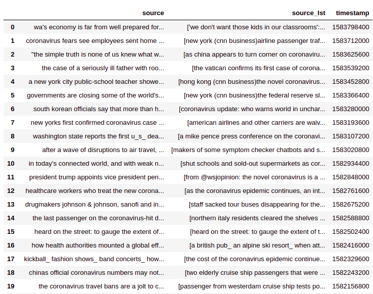
Every observation is the aggregation of news by day, we have the source which is the concatenation of all news into a string and the source_lst which is a list of the news of that interval.

The timestamp means the news happened in the interval from the prior timestamp to the current one :

interest_countries = ['China', 'Iran', 'Korea', 'Italy', 'France', 'Germany', 'Spain']for country in interest_countries:

df_news['count_news_' + country] = [len([text for text in daily_lst if country.lower() in text]) for daily_lst in df_news['source_lst']]df_news.reindex(index=df_news.index[::-1]).plot(x = 'timestamp', y = [col for col in df_news.columns if 'count' in col], figsize=(17,7), kind='area')

Let’s look at a word cloud from the last 20 days of news.

from os import path
from PIL import Image
from wordcloud import WordCloud, STOPWORDS, ImageColorGeneratorplt.figure()
plt.imshow(WordCloud(max_font_size=50, max_words=80, background_color="white").generate(' '.join([val for val in df['source'][0: 20]])), interpolation="bilinear")
plt.axis("off")
plt.show()plt.figure()
plt.imshow(WordCloud(max_font_size=50, max_words=80, background_color="white").generate(' '.join([val for val in df['source'][0: 20]])), interpolation="bilinear")
plt.axis("off")
plt.show()

Gather Financial and other Indicators

For this we can part from the Dow Jones Dataset and blend several others such as exchange rates (Yen, Euro, Pound), material prices (Crude Oil, Corn, Platinum, Tin), or stock (Coca Cola, Dow Jones).

action = 'API_getObservationsFromDataset'
        
parameters = {
 'token':'YOUR_TOKEN_HERE',
 'id_dataset':'5d4c14cd9516290b01c7d673', 'aggregate_in_time_interval':{"output":"avg","empty_intervals":"impute","time_interval_size":86400}, 'blends':[
        #Yen vs USD              
{"id_blend":"5d2495169516290b5fd2cee3","restriction":"None","blend_type":"ts","drop_features":[]},        # Euro Vs USD
{"id_blend":"5d4b3af1951629707cc1116b","restriction":"None","blend_type":"ts","drop_features":[]},        # Pound Vs USD              
{"id_blend":"5d4b3be1951629707cc11341","restriction":"None","blend_type":"ts","drop_features":[]},        # Corn Price    
{"id_blend":"5d4c23b39516290b01c7feea","restriction":"None","blend_type":"ts","drop_features":[]},        # CocaCola Price     
{"id_blend":"5d4c72399516290b02fe7359","restriction":"None","blend_type":"ts","drop_features":[]},        # Platinum price             
{"id_blend":"5d4ca1049516290b02fee837","restriction":"None","blend_type":"ts","drop_features":[]},        # Tin Price
{"id_blend":"5d4caa429516290b01c9dff0","restriction":"None","blend_type":"ts","drop_features":[]},        # Crude Oil Price
{"id_blend":"5d4c80bf9516290b01c8f6f9","restriction":"None","blend_type":"ts","drop_features":[]}],'date_filter':{"start_date":"2020-01-01T06:00:00.000Z","end_date":"2020-03-10T06:00:00.000Z"},
'consumption_confirmation':'on' 
}df = pd.read_json(json.dumps(OpenBlender.call(action, parameters)['sample']), convert_dates=False, convert_axes=False).sort_values('timestamp', ascending=False)
df.reset_index(drop=True, inplace=True)df.shape()
df.head()

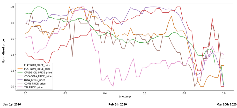
So now we have a single dataset with daily observations of prices blended by time. If we want to compare them, we better normalize them between 0 and 1, so that we can better appreciate the patterns:

# Lets compress all into the (0, 1) domain
df_compress = df.dropna(0).select_dtypes(include=['int16', 'int32', 'int64', 'float16', 'float32', 'float64']).apply(lambda x: (x - x.min()) / (x.max() - x.min()))
df_compress['timestamp'] = df['timestamp']# Now we select the columns that interest us
cols_of_interest = ['timestamp', 'PLATINUM_PRICE_price', 'CRUDE_OIL_PRICE_price', 'COCACOLA_PRICE_price', 'open', 'CORN_PRICE_price', 'TIN_PRICE_price', 'PLATINUM_PRICE_price']
df_compress = df_compress[cols_of_interest]
df_compress.rename(columns={'open':'DOW_JONES_price'}, inplace=True)# An now let's plot them
from matplotlib import pyplot as plt
fig, ax = plt.subplots(figsize=(17,7))
plt = df_compress.plot(x='timestamp', y =['PLATINUM_PRICE_price', 'CRUDE_OIL_PRICE_price', 'COCACOLA_PRICE_price', 'DOW_JONES_price', 'CORN_PRICE_price', 'TIN_PRICE_price', 'PLATINUM_PRICE_price'], ax=ax)

Blend all the data together

Now, we will align the COVID-19 confirmed cases, the coronavirus news and the economical indicators data into one single dataset blended by time.

# First the News Datasetaction = 'API_createDataset'parameters = { 
 'token':'YOUR_TOKEN_HERE',
 'name':'Coronavirus News',
 'description':'YOUR_DATASET_DESCRIPTION',
 'visibility':'private',
 'tags':[],
 'insert_observations':'on',
    'select_as_timestamp' : 'timestamp',
 'dataframe':df_news.to_json() 
}
        
OpenBlender.call(action, parameters)

# And now the Financial Indicatorsaction = 'API_createDataset'parameters = { 
 'token':'YOUR_TOKEN_HERE',
 'name':'Financial Indicators for COVID',
 'description':'YOUR_DATASET_DESCRIPTION',
 'visibility':'private',
 'tags':[],
 'insert_observations':'on',
 'select_as_timestamp' : 'timestamp',
 'dataframe':df_compress.to_json() 
}
        
OpenBlender.call(action, parameters)
And now we just pull the initial COVID-19 dataset and we blend the new datasets we created by replacing the “id_dataset”.

action = 'API_getObservationsFromDataset'# ANCHOR: 'COVID19 Confirmed Cases'
# BLENDS: 'Coronavirus News', 'Financial Indicators for COVID'
        
parameters = { 
 'token':'YOUR_TOKEN_HERE',
 'id_dataset':'5e6ac97595162921fda18076',
 'date_filter':{
               "start_date":"2020-01-01T06:00:00.000Z",
               "end_date":"2020-03-11T06:00:00.000Z"} ,
 
 },'filter_select' : {'feature' : 'countryregion', 'categories' : ['Italy']},'aggregate_in_time_interval':{"output":"avg","empty_intervals":"impute","time_interval_size":86400}, 'blends':[{"id_blend":"5e6b19ce95162921fda1b6a7","restriction":"None","blend_type":"ts","drop_features":[]},
            {"id_blend":"5e6b1aa095162921fda1b751","restriction":"None","blend_type":"ts","drop_features":[]}] 
}df = pd.read_json(json.dumps(OpenBlender.call(action, parameters)['sample']), convert_dates=False, convert_axes=False).sort_values('timestamp', ascending=False)
df.reset_index(drop=True, inplace=True)

Above we selected observations for ‘Italy’, aggregated by day in seconds (8640) and blended the new data.

df.head()

We have a dataset with the daily information of all the data